38 how to add percentage and category name data labels in excel

Pivot Chart Data Label Help Needed - Microsoft Community Open the Excel file with Pivot Chart and enabled with Data Labels> Click on the Labels displayed in the Chart> Right-click> Click Format Data Labels> Label Options> Number> In the Category, select the format as per your requirement. Here is the reference article: Change the format of data labels in a chart. Excel charts: add title, customize chart axis, legend and data labels To add a label to one data point, click that data point after selecting the series. Click the Chart Elements button, and select the Data Labels option. For example, this is how we can add labels to one of the data series in our Excel chart: For specific chart types, such as pie chart, you can also choose the labels location.

Chart.ApplyDataLabels method (Excel) | Microsoft Docs Syntax expression. ApplyDataLabels ( Type, LegendKey, AutoText, HasLeaderLines, ShowSeriesName, ShowCategoryName, ShowValue, ShowPercentage, ShowBubbleSize, Separator) expression A variable that represents a Chart object. Parameters Example This example applies category labels to series one on Chart1. VB Copy Charts ("Chart1").SeriesCollection (1).

How to add percentage and category name data labels in excel

How to show values in data labels of Excel ... - MrExcel Message Board 2) Move Value data series to 2nd Axis 3) Change Value data series Fill from Automatic to No Fill 4) Change 2nd Vertical Axis Labels to None 5) Add Data Labels to Value data series Hope this helps. Steve=True D dendres New Member Joined Aug 1, 2015 Messages 14 Aug 3, 2015 #3 Hi Steve=True, Thank you for the help. How to Add Data Bars in Excel? - EDUCBA In order to show only bars, you can follow the below steps. Step 1: Select the number range from B2:B11. Step 2: Go to Conditional Formatting and click on Manage Rules. Step 3: As shown below, double click on the rule. Step 4: Now, in the below window, select Show Bars Only and then click OK. Add or remove data labels in a chart - support.microsoft.com Add data labels to a chart Click the data series or chart. To label one data point, after clicking the series, click that data point. In the upper right corner, next to the chart, click Add Chart Element > Data Labels. To change the location, click the arrow, and choose an option.

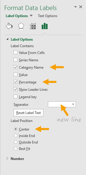
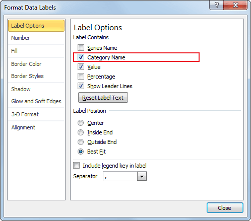
How to add percentage and category name data labels in excel. Display percentage values on pie chart in a paginated report ... To display percentage values as labels on a pie chart. Add a pie chart to your report. For more information, see Add a Chart to a Report (Report Builder and SSRS). On the design surface, right-click on the pie and select Show Data Labels. The data labels should appear within each slice on the pie chart. On the design surface, right-click on the ... How to add data labels from different column in an Excel chart? Right click the data series in the chart, and select Add Data Labels > Add Data Labels from the context menu to add data labels. 2. Click any data label to select all data labels, and then click the specified data label to select it only in the chart. 3. Column Chart That Displays Percentage Change or Variance - Excel Campus Select the chart, go to the Format tab in the ribbon, and select Series "Invisible Bar" from the drop-down on the left side. Choose Data Labels > More Options from the Elements menu. Select the Label Options sub menu in the Format Data Labels task pane. Click the Value from Cells checkbox. How to Add Data Labels to an Excel 2010 Chart - dummies On the Chart Tools Layout tab, click Data Labels→More Data Label Options. The Format Data Labels dialog box appears. You can use the options on the Label Options, Number, Fill, Border Color, Border Styles, Shadow, Glow and Soft Edges, 3-D Format, and Alignment tabs to customize the appearance and position of the data labels.

Change the format of data labels in a chart To get there, after adding your data labels, select the data label to format, and then click Chart Elements > Data Labels > More Options. To go to the appropriate area, click one of the four icons ( Fill & Line, Effects, Size & Properties ( Layout & Properties in Outlook or Word), or Label Options) shown here. Custom Chart Data Labels In Excel With Formulas Follow the steps below to create the custom data labels. Select the chart label you want to change. In the formula-bar hit = (equals), select the cell reference containing your chart label's data. In this case, the first label is in cell E2. Finally, repeat for all your chart laebls. excel - How can I add chart data labels with percentage? - Stack Overflow I want to add chart data labels with percentage by default with Excel VBA. Here is my code for creating the chart: Private Sub CommandButton2_Click() ActiveSheet.Shapes.AddChart.Select ActiveChart. How to show percentage in Excel - Ablebits.com To do this, open the Format Cells dialog either by pressing Ctrl + 1 or right-clicking the cell and selecting Format Cells… from the context menu. Make sure the Percentage category is selected and specify the desired number of decimal places in the Decimal places box. When done, click the OK button to save your settings.

How to show percentages in stacked column chart in Excel? Add percentages in stacked column chart 1. Select data range you need and click Insert > Column > Stacked Column. See screenshot: 2. Click at the column and then click Design > Switch Row/Column. 3. In Excel 2007, click Layout > Data Labels > Center . In Excel 2013 or the new version, click Design > Add Chart Element > Data Labels > Center. 4. Format Number Options for Chart Data Labels in Excel 2011 ... - Indezine Figure 1: Chart with Data Values added as Data Labels. Follow these steps to learn how to format the values used in Data Labels within Excel 2011: Select the chart -- then select the Charts tab which appears on the Ribbon, as shown highlighted in red within Figure 2. Within the Charts tab, click the Edit button (highlighted in blue within ... Count and Percentage in a Column Chart - ListenData Download the workbook. Steps to show Values and Percentage. 1. Select values placed in range B3:C6 and Insert a 2D Clustered Column Chart (Go to Insert Tab >> Column >> 2D Clustered Column Chart). See the image below. Insert 2D Clustered Column Chart. 2. In cell E3, type =C3*1.15 and paste the formula down till E6. How to Change Excel Chart Data Labels to Custom Values? First add data labels to the chart (Layout Ribbon > Data Labels) Define the new data label values in a bunch of cells, like this: Now, click on any data label. This will select "all" data labels. Now click once again. At this point excel will select only one data label.

Pie Chart: Survey results favorite ice cream flavor | Exceljet

Excel tutorial: How to use data labels When you check the box, you'll see data labels appear in the chart. If you have more than one data series, you can select a series first, then turn on data labels for that series only. You can even select a single bar, and show just one data label. In a bar or column chart, data labels will first appear outside the bar end.

CD: Pie Charts

Format Data Labels in Excel- Instructions - TeachUcomp, Inc. To do this, click the "Format" tab within the "Chart Tools" contextual tab in the Ribbon. Then select the data labels to format from the "Chart Elements" drop-down in the "Current Selection" button group. Then click the "Format Selection" button that appears below the drop-down menu in the same area.

Set up PivotTables using the PowerPivot add-on module

How to show data label in "percentage" instead of - Microsoft Community Select Format Data Labels Select Number in the left column Select Percentage in the popup options In the Format code field set the number of decimal places required and click Add. (Or if the table data in in percentage format then you can select Link to source.) Click OK Regards, OssieMac Report abuse 8 people found this reply helpful ·

Excel 3-D Pie charts - Microsoft Excel 2010

Add a DATA LABEL to ONE POINT on a chart in Excel All the data points will be highlighted. Click again on the single point that you want to add a data label to. Right-click and select ' Add data label '. This is the key step! Right-click again on the data point itself (not the label) and select ' Format data label '. You can now configure the label as required — select the content of ...

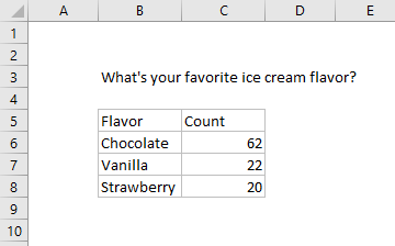
Pie Chart: Survey results favorite ice cream flavor | Exceljet

Solved: change data label to percentage - Power BI 06-08-2020 11:22 AM. Hi @MARCreading. pick your column in the Right pane, go to Column tools Ribbon and press Percentage button. do not hesitate to give a kudo to useful posts and mark solutions as solution. LinkedIn. View solution in original post. Message 2 of 7.

Excel 3-D Pie charts - Microsoft Excel 2016

How to Customize Your Excel Pivot Chart Data Labels - dummies The Data Labels command on the Design tab's Add Chart Element menu in Excel allows you to label data markers with values from your pivot table. When you click the command button, Excel displays a menu with commands corresponding to locations for the data labels: None, Center, Left, Right, Above, and Below. None signifies that no data labels ...

Excel Is Fun

Add data labels and callouts to charts in Excel 365 - EasyTweaks.com The steps that I will share in this guide apply to Excel 2021 / 2019 / 2016. Step #1: After generating the chart in Excel, right-click anywhere within the chart and select Add labels . Note that you can also select the very handy option of Adding data Callouts.

Pie Chart Examples | Types of Pie Charts in Excel with Examples

Multiple data labels (in separate locations on chart) Running Excel 2010 2D pie chart I currently have a pie chart that has one data label already set. The Pie chart has the name of the category and value as data labels on the outside of the graph. I now need to add the percentage of the section on the INSIDE of the graph, centered within the pie section. I'm aware that I could type in the percentages as text boxes, but I want this graph to ...

Share :