42 excel column chart labels
Add / Move Data Labels in Charts - Excel & Google Sheets Add and Move Data Labels in Google Sheets. Double Click Chart. Select Customize under Chart Editor. Select Series. 4. Check Data Labels. 5. Select which Position to move the data labels in comparison to the bars. Move and Align Chart Titles, Labels, Legends with the ... - Excel Campus Select the element in the chart you want to move (title, data labels, legend, plot area). On the add-in window press the "Move Selected Object with Arrow Keys" button. This is a toggle button and you want to press it down to turn on the arrow keys. Press any of the arrow keys on the keyboard to move the chart element.
Duplicate x-axis labels in column chart - Microsoft Community Duplicate x-axis labels in column chart. Hi! I am using Excel 2010 on a Windows 8.1 OP. I am trying to make histograms of air particulate concentration (y-axis) and weather data (x-axis). There are many instances where the value of weather data is repeated on different occasions. Rather than culminating all the spores that occur at a specific ...

Excel column chart labels
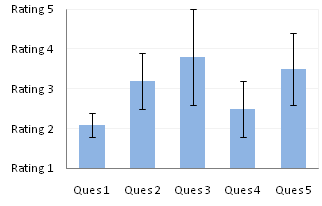
Data Labels in Excel Pivot Chart (Detailed Analysis) 7 Suitable Examples with Data Labels in Excel Pivot Chart Considering All Factors 1. Adding Data Labels in Pivot Chart 2. Set Cell Values as Data Labels 3. Showing Percentages as Data Labels 4. Changing Appearance of Pivot Chart Labels 5. Changing Background of Data Labels 6. Dynamic Pivot Chart Data Labels with Slicers 7. How to Add Two Data Labels in Excel Chart (with Easy Steps) Select any column representing demand units. Then right-click your mouse to bring the menu. After that, select Add Data Labels. Excel will add data labels for 2nd time. Step 4: Format Data Labels to Show Two Data Labels Here, I will discuss a remarkable feature of Excel charts. You can easily show two parameters in the data label. Text Labels on a Vertical Column Chart in Excel - Peltier Tech Right click on the new series, choose "Change Chart Type" ("Chart Type" in 2003), and select the clustered bar style. There are no Rating labels because there is no secondary vertical axis, so we have to add this axis by hand. On the Excel 2007 Chart Tools > Layout tab, click Axes, then Secondary Horizontal Axis, then Show Left to Right Axis.
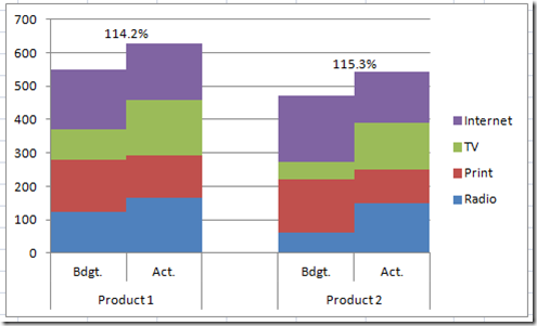
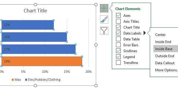
Excel column chart labels. How to Customize Your Excel Pivot Chart Data Labels - dummies The Data Labels command on the Design tab's Add Chart Element menu in Excel allows you to label data markers with values from your pivot table. When you click the command button, Excel displays a menu with commands corresponding to locations for the data labels: None, Center, Left, Right, Above, and Below. How to Add Labels to Show Totals in Stacked Column Charts in Excel The chart should look like this: 8. In the chart, right-click the "Total" series and then, on the shortcut menu, select Add Data Labels. 9. Next, select the labels and then, in the Format Data Labels pane, under Label Options, set the Label Position to Above. 10. While the labels are still selected set their font to Bold. 11. How to Use Cell Values for Excel Chart Labels - How-To Geek Select range A1:B6 and click Insert > Insert Column or Bar Chart > Clustered Column. The column chart will appear. We want to add data labels to show the change in value for each product compared to last month. Select the chart, choose the "Chart Elements" option, click the "Data Labels" arrow, and then "More Options." How to I rotate data labels on a column chart so that they are ... To change the text direction, first of all, please double click on the data label and make sure the data are selected (with a box surrounded like following image). Then on your right panel, the Format Data Labels panel should be opened. Go to Text Options > Text Box > Text direction > Rotate
Create a multi-level category chart in Excel - ExtendOffice Select the dots, click the Chart Elements button, and then check the Data Labels box. 23. Right click the data labels and select Format Data Labels from the right-clicking menu. 24. In the Format Data Labels pane, please do as follows. 24.1) Check the Value From Cells box; Combination Clustered and Stacked Column Chart in Excel Step 5 – Adjust the Series Overlap and Gap Width. In the chart, click the “Forecast” data series column. In the Format ribbon, click Format Selection.In the Series Options, adjust the Series Overlap and Gap Width sliders so that the “Forecast” data series does not overlap with the stacked column. Clustered Column Chart in Excel (In Easy Steps) - Excel Easy Click Clustered Column. Result: Note: only if you have numeric labels, empty cell A1 before you create the column chart. By doing this, Excel does not recognize the numbers in column A as a data series and automatically places these numbers on the horizontal (category) axis. After creating the chart, you can enter the text Year into cell A1 if ... Column Chart with Category Axis Labels Between Columns Right-click the series of blue dots, and choose Add Data Labels. Excel adds the default Y values (zeros) to the right of the markers. Format the labels so they are in the Below position, and so they show the X values instead of the Y values. Finally format the series of dots so they use no markers. And we're done.
Stacked Column Chart in Excel (examples) - EDUCBA This has been a guide to Stacked Column Chart in Excel. Here we discuss its uses and how to create Stacked Column Chart in Excel with excel examples and downloadable excel templates. You may also look at these useful functions in excel – Interactive Chart in Excel; Freeze Columns in Excel; Excel Clustered Column Chart; Excel Column Chart Column Chart In Excel | How to insert 2-D Column Chart in Excel | add ... Column Chart In Excel | How to insert 2-D Column Chart in Excel | add Title, Legend, data labels EtcChannel PlaylistsPythonhttps:// ... Column Chart in Excel | How to Make a Column Chart? (Examples) Column Chart in Excel. A column chart in Excel is a chart that is used to represent data in vertical columns. The height of the column represents the value for the specific data series in a chart. The column chart represents the comparison in the form of the column from left to right. If there is a single data series, it is easy to see the ... Add or remove data labels in a chart - support.microsoft.com Click the data series or chart. To label one data point, after clicking the series, click that data point. In the upper right corner, next to the chart, click Add Chart Element > Data Labels. To change the location, click the arrow, and choose an option. If you want to show your data label inside a text bubble shape, click Data Callout.
How-to Use Data Labels from a Range in an Excel Chart - Excel ...
Stagger long axis labels and make one label stand out in an Excel ... Select any column and press Ctrl+1 to open the Format Data Series task pane. In the Series Options, set the Series Overlap to 100%. You can also set the Gap Width to 50% to give the columns more presence on the chart. Use the "+" chart skittle to remove the legend and gridlines. Add a chart title if desired. The chart will now look like this.

excel - VBA Change Data Labels on a Stacked Column chart from ...
Edit titles or data labels in a chart - support.microsoft.com On a chart, click the label that you want to link to a corresponding worksheet cell. On the worksheet, click in the formula bar, and then type an equal sign (=). Select the worksheet cell that contains the data or text that you want to display in your chart. You can also type the reference to the worksheet cell in the formula bar.

Excel: How to create a dual axis chart with overlapping bars ...
How to add data labels from different column in an Excel chart? Right click the data series in the chart, and select Add Data Labels > Add Data Labels from the context menu to add data labels. 2. Click any data label to select all data labels, and then click the specified data label to select it only in the chart. 3.

Use this trick in Excel to control long category labels in ...
How to Make a Column Chart in Excel: A Guide to Doing it Right The data is arranged with the labels in the first column and the values in the second column. Nice and simple. The chart will have no problem interpreting this layout. ... we saw how to make a column chart in Excel and perform some typical formatting changes. And then explored some of the other column chart types available in Excel, and why ...

Two-Level Axis Labels (Microsoft Excel)
Chart Data Labels > Alignment > Label Position: Outsid Go to the Chart menu > Chart Type. Verify the sub-type. If it's stacked column (the option in the first row that is second from the left), this is why Outside End is not an option for label position. While still in the Chart Type dialog box, you can change the sub-type to clustered column (the option in the first row that is first on the left).

Adding rich data labels to charts in Excel 2013 | Microsoft ...
Excel Custom Chart Labels • My Online Training Hub Note: Excel 2013 onward also requires this step if you have more than one series you want to position your labels above. Step 1: Select cells A26:D38 and insert a column Chart. Step 2: Select the Max series and plot it on the Secondary Axis: double click the Max series > Format Data Series > Secondary Axis: Step 3: Insert labels on the Max ...

How to Add Axis Labels to a Chart in Excel | CustomGuide
How to Add Total Data Labels to the Excel Stacked Bar Chart Apr 03, 2013 · For stacked bar charts, Excel 2010 allows you to add data labels only to the individual components of the stacked bar chart. The basic chart function does not allow you to add a total data label that accounts for the sum of the individual components. Fortunately, creating these labels manually is a fairly simply process.

Custom Data Labels with Colors and Symbols in Excel Charts ...
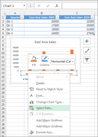
How to Directly Label Stacked Column Charts in Excel - simplexCT On the worksheet, right-click the chart and then, on the shortcut menu, click Select Data. 4. Next, In the Select Data Source dialog box, click on the Add button under Legend Entries (Series). 5. In the Edit Series dialog box, type "Labels" in the Series name edit box and refer to cell B13 in the Series values edit box as per the below screenshot:

How to Add Data Labels to an Excel 2010 Chart - dummies
How to Add Axis Labels in Excel Charts - Step-by-Step (2022) - Spreadsheeto Left-click the Excel chart. 2. Click the plus button in the upper right corner of the chart. 3. Click Axis Titles to put a checkmark in the axis title checkbox. This will display axis titles. 4. Click the added axis title text box to write your axis label. Or you can go to the 'Chart Design' tab, and click the 'Add Chart Element' button ...

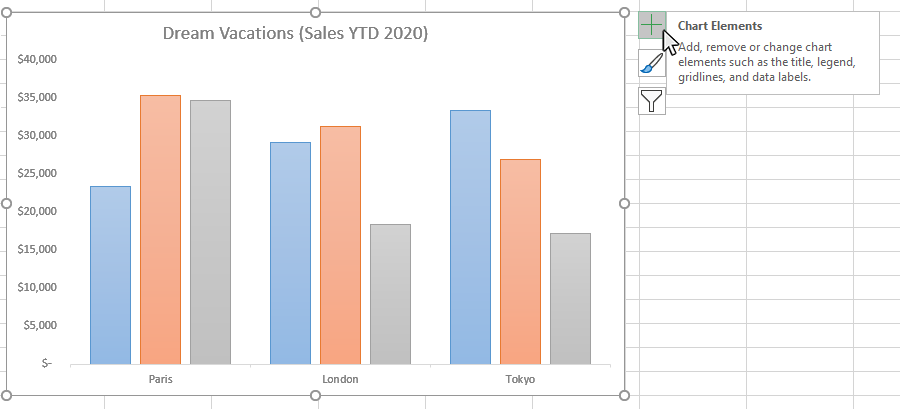
How to Add and Remove Chart Elements in Excel
Adding Labels to Column Charts | Online Excel Training | Kubicle To add data labels, just right-click on a data series and click add data labels. To see the data labels clearly, I'll need to select them and change their color to white. The data labels are determined by the vertical axis of your chart. Currently, the vertical axis shows millions, therefore, my data labels are shown in millions as well.
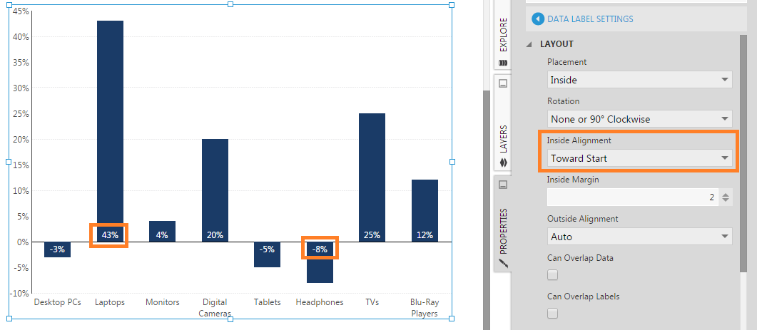
Aligning data point labels inside bars | How-To | Data ...
How to Insert Axis Labels In An Excel Chart | Excelchat We will go to Chart Design and select Add Chart Element Figure 6 - Insert axis labels in Excel In the drop-down menu, we will click on Axis Titles, and subsequently, select Primary vertical Figure 7 - Edit vertical axis labels in Excel Now, we can enter the name we want for the primary vertical axis label.

Moving the axis labels when a PowerPoint chart/graph has both ...
Excel Charts - Aesthetic Data Labels - tutorialspoint.com A Leader line is a line that connects a data label and its associated data point. It is helpful when you have placed a data label away from a data point. All chart types with data labels have this functionality from Excel 2013 onwards. In earlier versions of Excel, only Pie charts had this functionality. Step 1 − Click the data label.
How-to Add Centered Labels Above an Excel Clustered Stacked ...
Dynamically Label Excel Chart Series Lines - My Online Training Hub Step 1: Duplicate the Series. The first trick here is that we have 2 series for each region; one for the line and one for the label, as you can see in the table below: Select columns B:J and insert a line chart (do not include column A). To modify the axis so the Year and Month labels are nested; right-click the chart > Select Data > Edit the ...
/simplexct/images/Fig2-79394.jpg)
How to Create a Bar Chart With Labels Above Bars in Excel
Column Chart with Primary and Secondary Axes - Peltier Tech Oct 28, 2013 · Plot data in clustered column chart (Chart 1). Assign Sec 1 & Sec 2 to secondary axis (Chart 2). Set primary Y axis scale to 0 min and 6 max, set secondary Y axis scale to -30 min and +30 max (Chart 3). Use custom number format [<=3]0;;; for primary axis tick labels, use custom number format 0;;0; for secondary axis tick labels (Chart 4).
Excel Data Labels: How to add totals as labels to a stacked ...
how to align x-axis labels in column chart? - MrExcel Message Board The Excel help page "Change the display of chart axes" ( click here) [1] explains: "You can also change the horizontal alignment of axis labels, by right-clicking the axis, and then click Align Left Button image, Center Button image, or Align Right Button image on the Mini toolbar."

Custom Excel Chart Label Positions • My Online Training Hub
Text Labels on a Vertical Column Chart in Excel - Peltier Tech Right click on the new series, choose "Change Chart Type" ("Chart Type" in 2003), and select the clustered bar style. There are no Rating labels because there is no secondary vertical axis, so we have to add this axis by hand. On the Excel 2007 Chart Tools > Layout tab, click Axes, then Secondary Horizontal Axis, then Show Left to Right Axis.

Is there a way to show different data labels in a bar chart ...
How to Add Two Data Labels in Excel Chart (with Easy Steps) Select any column representing demand units. Then right-click your mouse to bring the menu. After that, select Add Data Labels. Excel will add data labels for 2nd time. Step 4: Format Data Labels to Show Two Data Labels Here, I will discuss a remarkable feature of Excel charts. You can easily show two parameters in the data label.

How to group (two-level) axis labels in a chart in Excel?
Data Labels in Excel Pivot Chart (Detailed Analysis) 7 Suitable Examples with Data Labels in Excel Pivot Chart Considering All Factors 1. Adding Data Labels in Pivot Chart 2. Set Cell Values as Data Labels 3. Showing Percentages as Data Labels 4. Changing Appearance of Pivot Chart Labels 5. Changing Background of Data Labels 6. Dynamic Pivot Chart Data Labels with Slicers 7.
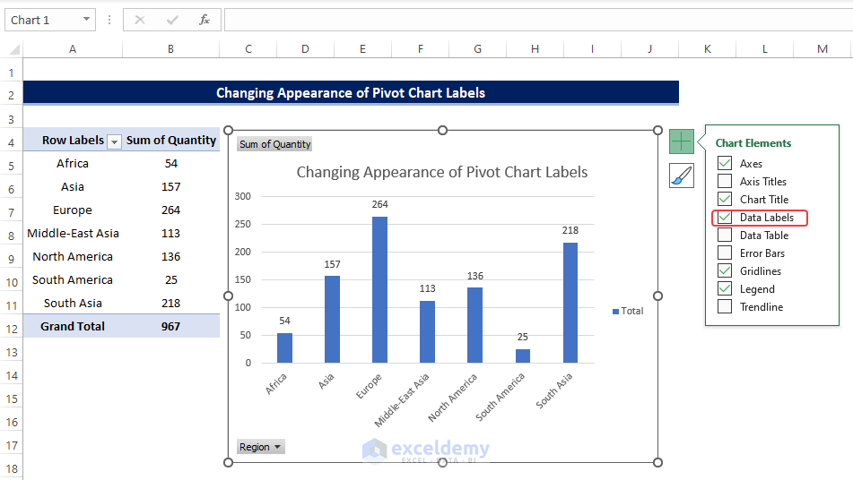
Data Labels in Excel Pivot Chart (Detailed Analysis) - ExcelDemy
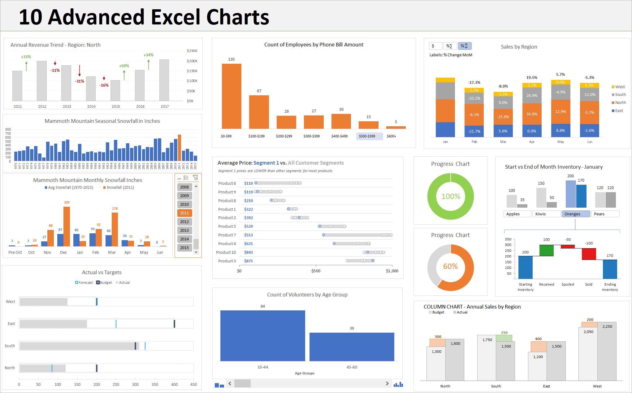
10 Advanced Excel Charts - Excel Campus

Custom Excel Chart Label Positions • My Online Training Hub

How to Customize for a GREAT-Looking Excel Chart

Aligning data point labels inside bars | How-To | Data ...
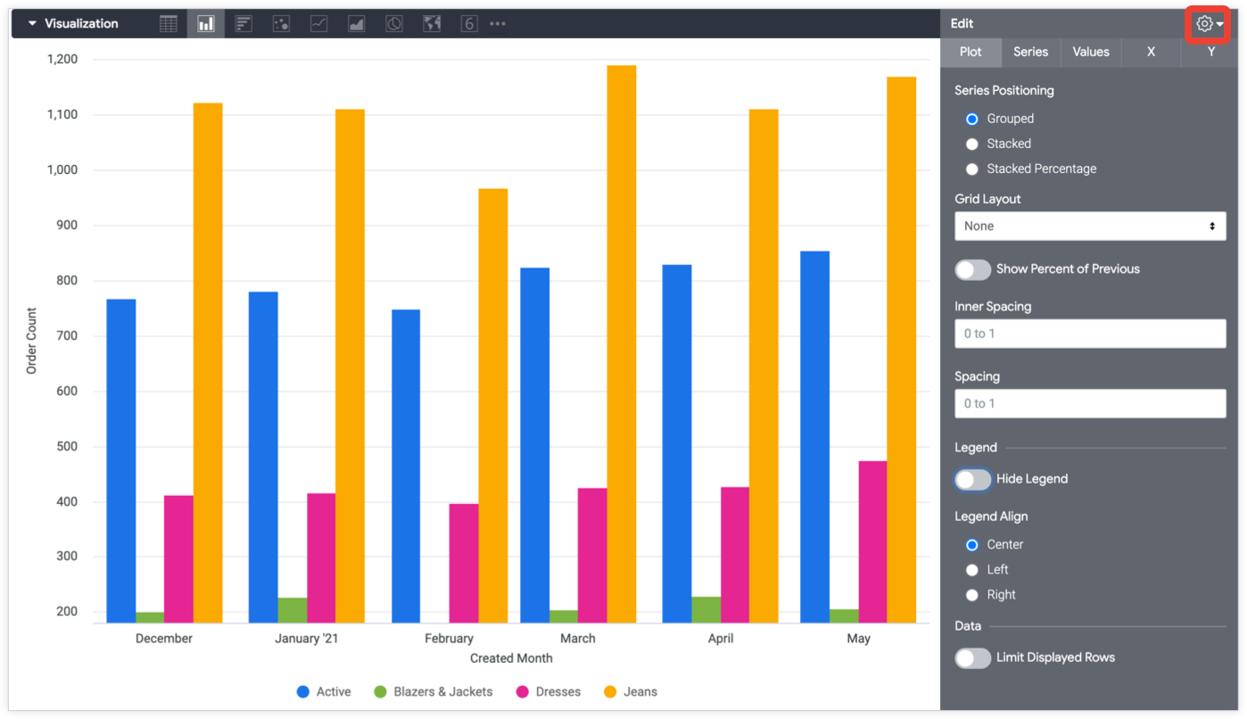
Column chart options | Looker | Google Cloud
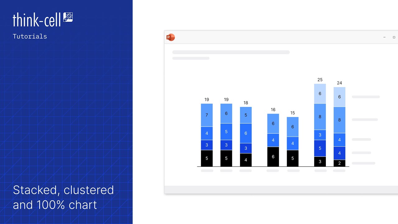
How to create column charts, line charts and area charts in ...

Custom data labels in a chart
Move and Align Chart Titles, Labels, Legends with the Arrow ...
EXCEL Charts: Column, Bar, Pie and Line
/simplexct/BlogPic-3a631.png)
How to Directly Label Stacked Column Charts in Excel
Change axis labels in a chart
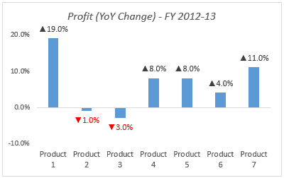
Color Negative Chart Data Labels in Red with downward arrow

How to add data labels from different column in an Excel chart?
How-to Center Excel Clustered Chart Columns Over Horizontal ...
Text Labels on a Vertical Column Chart in Excel - Peltier Tech
How to Add Axis Labels to a Chart in Excel - Business ...

Labeling a Stacked Column Chart in Excel - PolicyViz

How to Add Data Labels to your Excel Chart in Excel 2013

excel - How to show series-Legend label name in data labels ...

Dynamically Label Excel Chart Series Lines • My Online ...
Excel Bar Chart with Vertical Line • My Online Training Hub
Changing Y-Axis Label Width (Microsoft Excel)

How to Change Excel Chart Data Labels to Custom Values?
Post a Comment for "42 excel column chart labels"