43 format data labels excel 2016

How to Format Excel Pivot Table - Contextures Excel Tips 22.06.2022 · Copy a Custom Style in Excel 2016 or Later. In Excel 2016, the custom pivot table style is not copied, if you use the above technique to copy and paste a pivot table. I found a different way to copy the custom style, and this method also works in Excel 2013. In Excel 2016, follow these steps to copy a custom style into a different workbook: Excel 2016 Waterfall Chart - How to use, advantages and ... - XelPlus To use the new Excel 2016 Waterfall Chart, ... Looking at the options that we have for the data labels under the Format Data Labels > Label Options > Label Position, we can position the labels on the Outside End, Inside End, Center, and Inside Base. But you will not find an option to place the labels Always on top.

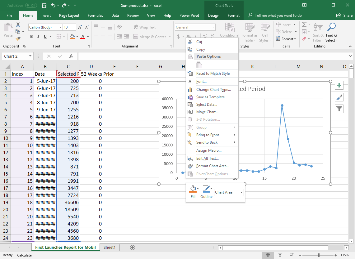
chandoo.org › wp › change-data-labels-in-chartsHow to Change Excel Chart Data Labels to Custom Values? May 05, 2010 · Now, click on any data label. This will select “all” data labels. Now click once again. At this point excel will select only one data label. Go to Formula bar, press = and point to the cell where the data label for that chart data point is defined. Repeat the process for all other data labels, one after another. See the screencast.

Format data labels excel 2016

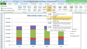
How to Add Total Data Labels to the Excel Stacked Bar Chart 03.04.2013 · Step 5: Right click your new data labels and format them so that their label position is “Above”; also make the labels bold and increase the font size . Step 6: Right click the line, select “Format Data Series”; in the Line Color menu, select “No line” Step 7: Delete the “Total” data series label within the legend. Categories Excel, Visual Design Tags charts, hacks ... Edit titles or data labels in a chart - support.microsoft.com You can also place data labels in a standard position relative to their data markers. Depending on the chart type, you can choose from a variety of positioning options. On a chart, do one of the following: To reposition all data labels for an entire data series, click a data label once to select the data series. Add or remove data labels in a chart - support.microsoft.com Click Label Options and under Label Contains, pick the options you want. Use cell values as data labels You can use cell values as data labels for your chart. Right-click the data series or data label to display more data for, and then click Format Data Labels. Click Label Options and under Label Contains, select the Values From Cells checkbox.

Format data labels excel 2016. Excel 2016: Formatting Cells - GCFGlobal.org Select the cell (s) you want to modify. Click the Bold ( B ), Italic ( I ), or Underline ( U) command on the Home tab. In our example, we'll make the selected cells bold. The selected style will be applied to the text. You can also press Ctrl+B on your keyboard to make selected text bold, Ctrl+I to apply italics, and Ctrl+U to apply an underline. How to Create Mailing Labels in Excel | Excelchat Step 1 - Prepare Address list for making labels in Excel First, we will enter the headings for our list in the manner as seen below. First Name Last Name Street Address City State ZIP Code Figure 2 - Headers for mail merge Tip: Rather than create a single name column, split into small pieces for title, first name, middle name, last name. Excel 2016: "Value from Cells" box under Format Data Labels Missing To label the point, please select the chart > Design > Add Chart Element > Data Labels. I still can see it by my side. See: To check if the issue is related to the Office program itself, you can run Office online repair. If you still meet issue, please tell us in which step you stuck. And provide us information below: 1. How to create Custom Data Labels in Excel Charts - Efficiency 365 Right click on any data label and choose the callout shape from Change Data Label Shapes option. Now adjust each data label as required to avoid overlap. Put solid fill color in the labels Finally, click on the chart (to deselect the currently selected label) and then click on a data label again (to select all data labels).

support.microsoft.com › en-us › officeEdit titles or data labels in a chart - support.microsoft.com To reposition all data labels for an entire data series, click a data label once to select the data series. To reposition a specific data label, click that data label twice to select it. This displays the Chart Tools , adding the Design , Layout , and Format tabs. docs.microsoft.com › office-file-format-referenceFile format reference for Word, Excel, and PowerPoint ... Sep 30, 2021 · The macro-enabled file format for an Excel template for Excel 2019, Excel 2016, Excel 2013, Excel 2010, and Office Excel 2007. Stores VBA macro code or Excel 4.0 macro sheets (.xlm). .xltx : Excel Template : The default file format for an Excel template for Excel 2019, Excel 2016, Excel 2013, Excel 2010, and Office Excel 2007. › charts › dynamic-chart-dataCreate Dynamic Chart Data Labels with Slicers - Excel Campus Feb 09, 2016 · Step 3: Use the TEXT Function to Format the Labels. Typically a chart will display data labels based on the underlying source data for the chart. In Excel 2013 a new feature called “Value from Cells” was introduced. This feature allows us to specify the a range that we want to use for the labels. Excel 2016 VBA Display every nth Data Label on Chart Click on the bar you want to labeled twice before Add Data Labels. Click on the label, then right click and select Format Data Labels. Check the Category Name and uncheck Value. A little research before asking can save you a lot of time. Share Improve this answer Follow answered Nov 7, 2017 at 13:15 user8753746user8753746

Excel 2016 Tutorial Formatting Data Labels Microsoft Training ... - YouTube FREE Course! Click: about Formatting Data Labels in Microsoft Excel at . A clip from Mastering Excel M... How to Print Labels from Excel - Lifewire 05.04.2022 · How to Print Labels From Excel . You can print mailing labels from Excel in a matter of minutes using the mail merge feature in Word. With neat columns and rows, sorting abilities, and data entry features, Excel might be the perfect application for entering and storing information like contact lists.Once you have created a detailed list, you can use it with other … Change the format of data labels in a chart Data labels make a chart easier to understand because they show details about a data series or its individual data points. For example, in the pie chart below, without the data labels it would be difficult to tell that coffee was 38% of total sales. You can format the labels to show specific labels elements like, the percentages, series name, or category name. Excel 2016: How to Format Data and Cells - UniversalClass.com To do this, go to the Format Cells dialogue box again, and click Custom n the category column. In the Type list, select the format that you want to customize. As you can see in the snapshot above, we chose the currency format. Now go to the Type field and customize the format by entering the format you want to use. Click OK when you're finished.

Change Horizontal Axis Values in Excel 2016 - AbsentData

3D maps excel 2016 add data labels - excelforum.com Re: 3D maps excel 2016 add data labels I don't think there are data labels equivalent to that in a standard chart. The bars do have a detailed tool tip but that required the map to be interactive and not a snapped picture. You could add annotation to each point. Select a stack and right click to Add annotation. Cheers Andy

Create Dynamic Chart Data Labels with Slicers - Excel Campus

Create Dynamic Chart Data Labels with Slicers - Excel Campus 09.02.2016 · Step 5: Setup the Data Labels. The next step is to change the data labels so they display the values in the cells that contain our CHOOSE formulas. As I mentioned before, we can use the “Value from Cells” feature in Excel 2013 or 2016 to make this easier. You basically need to select a label series, then press the Value from Cells button in ...

How to Create an Ogive Graph in Excel - Automate Excel

Format Data Labels in Excel- Instructions - TeachUcomp, Inc. To format data labels in Excel, choose the set of data labels to format. To do this, click the "Format" tab within the "Chart Tools" contextual tab in the Ribbon. Then select the data labels to format from the "Chart Elements" drop-down in the "Current Selection" button group.

Show Trend Arrows in Excel Chart Data Labels

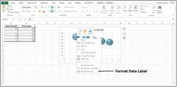
How to hide zero data labels in chart in Excel? - ExtendOffice If you want to hide zero data labels in chart, please do as follow: 1. Right click at one of the data labels, and select Format Data Labels from the context menu. See screenshot: 2. In the Format Data Labels dialog, Click Number in left pane, then select Custom from the Category list box, and type #"" into the Format Code text box, and click Add button to add it to Type list box.

How to Print Address Labels From Excel? (with Examples)

File format reference for Word, Excel, and PowerPoint - Deploy … 30.09.2021 · The binary file format for Excel 2019, Excel 2016, Excel 2013, and Excel 2010 and Office Excel 2007. This is a fast load-and-save file format for users who need the fastest way possible to load a data file. Supports VBA projects, Excel 4.0 macro sheets, and all the new features that are used in Excel. But, this is not an XML file format and is therefore not optimal …

Lesson 1: Getting Started with Microsoft Excel

How to create waterfall chart in Excel 2016, 2013, 2010 25.07.2014 · The Format Data Series pane immediately appears to the right of your worksheet in Excel 2013 / 2016. Click on the Fill & Line icon. Select No fill in the Fill section and No line in the Border section. When the blue columns become invisible, just delete Base from the chart legend to completely hide all the traces of the Base series. Step 5. Format Excel bridge chart. Let's …

Automatically update data labels on Excel chart (Excel 2016) - Stack Overflow

Excel tutorial: How to use data labels Generally, the easiest way to show data labels to use the chart elements menu. When you check the box, you'll see data labels appear in the chart. If you have more than one data series, you can select a series first, then turn on data labels for that series only. You can even select a single bar, and show just one data label.

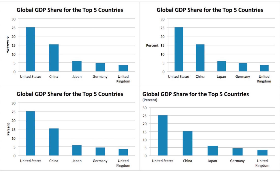
Where to Position the Y-Axis Label - PolicyViz

› excel-pivot-table-formatHow to Format Excel Pivot Table - Contextures Excel Tips Jun 22, 2022 · Copy a Custom Style in Excel 2016 or Later. In Excel 2016, the custom pivot table style is not copied, if you use the above technique to copy and paste a pivot table. I found a different way to copy the custom style, and this method also works in Excel 2013. In Excel 2016, follow these steps to copy a custom style into a different workbook:

ExcelQuickPages

Advanced Excel - Richer Data Labels - tutorialspoint.com Step 2 − Click on Change Data Label Shapes. Step 3 − Choose the shape you want. Resize a Data Label Step 1 − Click on the data label. Step 2 − Drag it to the size you want. Alternatively, you can click on Size & Properties icon in the Format Data Labels task pane and then choose the size options. Add a Field to a Data Label

How to Export a QuickBooks Report to Microsoft Excel | Webucator

How to Add Data Labels to an Excel 2010 Chart - dummies Excel provides several options for the placement and formatting of data labels. Use the following steps to add data labels to series in a chart: Click anywhere on the chart that you want to modify. On the Chart Tools Layout tab, click the Data Labels button in the Labels group. A menu of data label placement options appears: None: The default ...

32 How To Label Series In Excel - Labels 2021

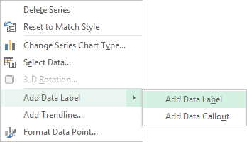
How to add data labels from different column in an Excel chart? This method will introduce a solution to add all data labels from a different column in an Excel chart at the same time. Please do as follows: 1. Right click the data series in the chart, and select Add Data Labels > Add Data Labels from the context menu to add data labels. 2. Right click the data series, and select Format Data Labels from the ...

How to Add Data Labels in Excel - Excelchat | Excelchat

How to Change Excel Chart Data Labels to Custom Values? 05.05.2010 · Now, click on any data label. This will select “all” data labels. Now click once again. At this point excel will select only one data label. Go to Formula bar, press = and point to the cell where the data label for that chart data point is defined. Repeat the process for all other data labels, one after another. See the screencast.

Create Custom Data Labels in Excel Charts - YouTube

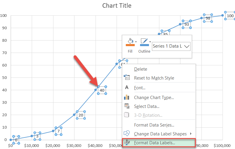
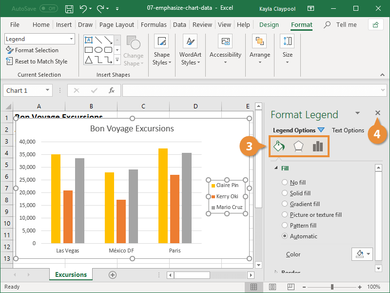
support.microsoft.com › en-us › officeChange the format of data labels in a chart To get there, after adding your data labels, select the data label to format, and then click Chart Elements > Data Labels > More Options. To go to the appropriate area, click one of the four icons ( Fill & Line , Effects , Size & Properties ( Layout & Properties in Outlook or Word), or Label Options ) shown here.

Creating a chart with dynamic labels - Microsoft Excel 2013

Formatting in Excel (Examples) | How to Format Data in Excel? - EDUCBA Now we will do data formatting in excel and will make this data in a presentable format. First, select the header field and make it bold. Select the whole data and choose the "All Border option" under the border. Now select the header field and make the thick border by selecting the "Thick box border" under the border.

Format Data Labels in Excel- Instructions - TeachUcomp, Inc.

Values From Cell: Missing Data Labels Option in Excel 2016? (Mac) For a new thread (1st post), scroll to Manage Attachments, otherwise scroll down to GO ADVANCED, click, and then scroll down to MANAGE ATTACHMENTS and click again. Now follow the instructions at the top of that screen. New Notice for experts and gurus:

Microsoft Excel Tutorials: The Chart Layout Panels

Open Excel 97/2003 xls files in versions 2016/365/2019 Now the default save format option for Excel documents will be as a xls file. Voi’la you are able to open older Excel versions in Excel 2016. Converting Excel workbooks with VBA Macros or Python scripts. If you have a very significant amount of documents you would like to convert, you could potentially automate the entire task.

Format Excel Chart Data | CustomGuide

Excel Charts - Aesthetic Data Labels - tutorialspoint.com To format a single data label −. Step 1 − Click twice any data label you want to format. Step 2 − Right-click that data label and then click Format Data Label. Alternatively, you can also click More Options in data labels options to display on the Format Data Label task pane. There are many formatting options for data labels in the format ...

Share :