40 row labels in excel pivot table

How to Move Excel Pivot Table Labels Quick Tricks - Contextures Excel Tips Jul 12, 2021 · Move Pivot Table Labels. This short video shows 3 ways to manually move the labels in a pivot table, and the written instructions are below the video. Drag a Label. Use Menu Commands. Type over a Label. Drag Labels to New Position. To move a pivot table label to a different position in the list, you can drag it: Click on the label that you want ... Excel Pivot Table Subtotals - Contextures Excel Tips Feb 01, 2022 · In the pivot table shown below, Service is in the Row Labels area, Lead Tech is in the Column Labels area, and Labor Cost is in the Values area. Because Service is the only field in the Row Labels area, it has no subtotal. Multiple Row Fields. When you add another field to the Row Labels area, a subtotal is automatically created for the first ...

How to Insert a Blank Row in Excel Pivot Table | MyExcelOnline Jan 17, 2021 · STEP 1: Click any cell in the Pivot Table. STEP 2: Go to Design > Blank Rows. STEP 3: You will need to click on the Blank Rows button and select Insert Blank Line After Each Item. NB: For this to work you will need at least two Pivot Table Items in the Rows Labels. You then get the following Pivot Table report:

Row labels in excel pivot table

Pivot table - Wikipedia Pivot tables are not created automatically. For example, in Microsoft Excel one must first select the entire data in the original table and then go to the Insert tab and select "Pivot Table" (or "Pivot Chart"). The user then has the option of either inserting the pivot table into an existing sheet or creating a new sheet to house the pivot table. How to reverse a pivot table in Excel? - ExtendOffice 5. Now a new pivot table is created, and double click last cell at the right down corner of new Pivot table, then a new table is created in a new worksheet. See screenshots: iv> 6. Then create a new pivot table based on this new table. Select the whole new table, and click Insert > PivotTable > PivotTable. 7. MS Excel 2016: How to Create a Pivot Table - TechOnTheNet Steps to Create a Pivot Table. To create a pivot table in Excel 2016, you will need to do the following steps: Before we get started, we first want to show you the data for the pivot table. In this example, the data is found on Sheet1. Highlight the cell where you'd like to create the pivot table. In this example, we've selected cell A1 on Sheet2.

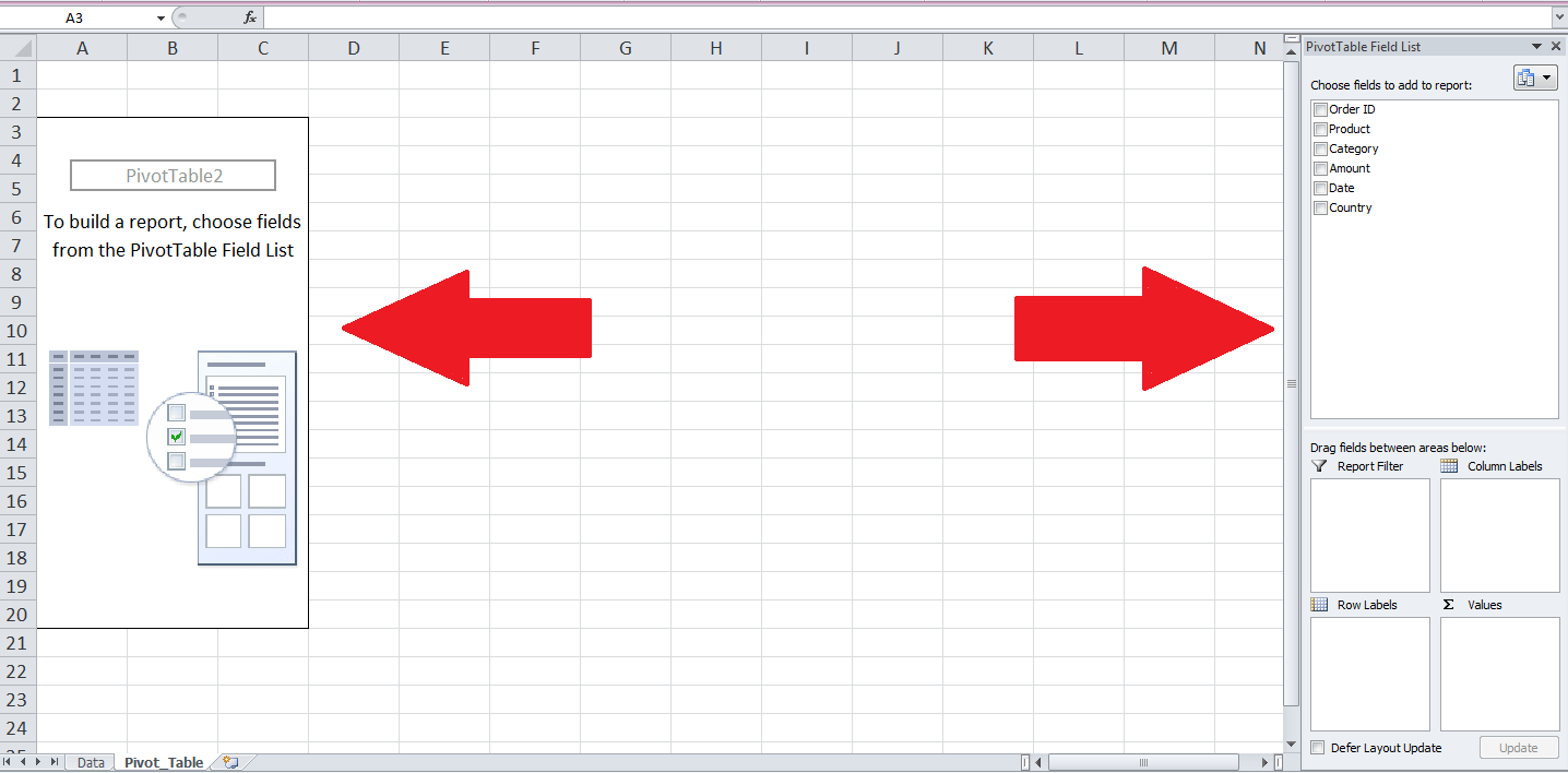
Row labels in excel pivot table. How to Create Excel Pivot Table (Includes practice file) 28/06/2022 · The area to the left results from your selections from [1] and [2]. You’ll see that the only difference I made in the last pivot table was to drag the AGE GROUP field underneath the PRECINCT field in the Row Labels quadrant. How to Create Excel Pivot Table. There are several ways to build a pivot table. How to Create Excel Pivot Table (Includes practice file) Jun 28, 2022 · The area to the left results from your selections from [1] and [2]. You’ll see that the only difference I made in the last pivot table was to drag the AGE GROUP field underneath the PRECINCT field in the Row Labels quadrant. How to Create Excel Pivot Table. There are several ways to build a pivot table. How to Replace Blank Cells with Zeros in Excel Pivot Tables Excel Pivot Tables has an option to quickly replace blank cells with zeroes. Here is how to do this: Right-click any cell in the Pivot Table and select Pivot Table Options. In Pivot Table Options Dialogue Box, within the Layout & Format tab, make sure that the For Empty cells show option is checked, and enter 0 in the field next to it. Excel: How to Filter Data in Pivot Table Using “Greater Than” May 05, 2022 · Often you may want to filter values in a pivot table in Excel using a “Greater Than” filter. Fortunately this is easy to do using the Value Filters dropdown menu within the Row Labels column of a pivot table. The following example shows exactly how to do so. Example: Filter Data in Pivot Table Using “Greater Than”

MS Excel 2016: How to Create a Pivot Table - TechOnTheNet Steps to Create a Pivot Table. To create a pivot table in Excel 2016, you will need to do the following steps: Before we get started, we first want to show you the data for the pivot table. In this example, the data is found on Sheet1. Highlight the cell where you'd like to create the pivot table. In this example, we've selected cell A1 on Sheet2. How to reverse a pivot table in Excel? - ExtendOffice 5. Now a new pivot table is created, and double click last cell at the right down corner of new Pivot table, then a new table is created in a new worksheet. See screenshots: iv> 6. Then create a new pivot table based on this new table. Select the whole new table, and click Insert > PivotTable > PivotTable. 7. Pivot table - Wikipedia Pivot tables are not created automatically. For example, in Microsoft Excel one must first select the entire data in the original table and then go to the Insert tab and select "Pivot Table" (or "Pivot Chart"). The user then has the option of either inserting the pivot table into an existing sheet or creating a new sheet to house the pivot table.

Pivot Table Row Labels Side By Side | Decorations I Can Make