44 add data labels to waterfall chart

How to Create Waterfall Chart in Excel? (Step by Step Examples) The data will look like this: Now, select cells A2:E16 and click on "Charts.". Click on "Column" and plot a Stacked Column chart in excel. The chart will look like this. Now, you can change the color of the "Base" columns to transparent or no fill. The chart will turn into a waterfall chart, as shown below. How to add Data markers in Waterfall chart in Plotly I am trying to plot waterfall chart with the following code. The only issue I am facing currently is the data marker which is not at the correct place. I want the data marker to be just below the end of each bar. Attached the screenshot of the waterfall chart. So for the first bar, I need the data marker to be just below the end of red bar.

Waterfall Chart in Excel (Examples) | How to Create Waterfall Chart? Select the blue bricks and right-click and select the option "Add Data Labels". Then you will get the values on the bricks; for better visibility, change the brick color to light blue. Double click on the "chart title" and change to the waterfall chart. If you observe, we can see both monthly sales and accumulated sales in the singles chart.

Add data labels to waterfall chart

How to Create a Waterfall Chart Template | GoCardless Select the data you want to highlight, including row and column headers. Go to the 'Insert' tab, click on 'Column Charts', and then select the 'Stacked Chart' option. Step 3: Convert the stacked chart to a waterfall chart Now you can convert the stacked chart to a waterfall chart format. To do this, you'll need to hide the 'Base' series from view. Excel Waterfall Chart: How to Create One That Doesn't Suck - Zebra BI Ideally, you would create a waterfall chart the same way as any other Excel chart: (1) click inside the data table, (2) click in the ribbon on the chart you want to insert. ... in Excel 2016 Microsoft decided to listen to user feedback and introduced 6 highly requested charts in Excel 2016, including a built-in Excel waterfall chart. Not able to add data label in waterfall chart using ggplot2 I am trying to plot waterfall chart using ggplot2. When I am placing the data labels it is not putting in the right place. Below is the code I am using dataset <- data.frame(TotalHeadcount =...

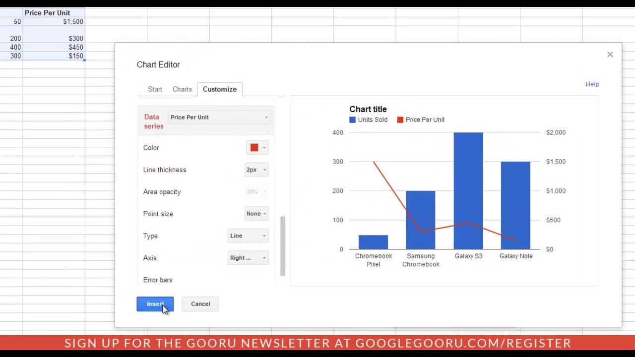
Add data labels to waterfall chart. Excel Waterfall Charts • My Online Training Hub For Excel 2007 or 2010 users there is no easy way to add labels. Adding labels to the chart will result in a mess which you have to tidy up. To tidy them up select each label box with 2 single left-clicks, then click in the formula bar and type = then click on the cell containing the label value in the chart source data table and press ENTER. Waterfall charts - Google Docs Editors Help Customize a waterfall chart. On your computer, open a spreadsheet in Google Sheets. Double-click the chart you want to change. At the right, click Customize. Chart style: Change how the chart looks, or add and edit connector lines. Chart & axis titles: Edit or format title text. Series: Change column colors, add and edit subtotals and data labels. How to Create a Waterfall Chart in Excel? - Spreadsheet Planet Now that the data is ready, let us use it to create a Waterfall Chart. Here are the steps: Select your data (cells A1:B7). Click on the Insert tab. Under the 'Charts' group, select the Waterfall Chart dropdown. Click on the Waterfall Chart from the menu that appears. Your Waterfall Chart should now appear in your worksheet. Introducing the Waterfall chart—a deep dive to a more streamlined chart ... To start, select your data and then under the Insert tab click the Recommended Charts button. The list of recommended charts is displayed. Select the Waterfall recommendation to preview the chart with your selected data. The All Charts tab allows direct insertion of Waterfall charts.

How to Create a Waterfall Chart in Excel - Automate Excel Right-click on any column and select "Add Data Labels." Immediately, the default data labels tied to the helper values will be added to the chart: But that is not exactly what we are looking for. To work around the issue, manually replace the default labels with the custom values you prepared beforehand. Double-click the data label you want ... Use a screen reader to add a title, data labels, and a legend to a ... Add a legend to a chart. Legends help you to quickly understand data relationships in a chart. For example, in your monthly budget worksheet, when you create a bar chart comparing projected costs with actual costs per expense category, a legend helps you to quickly identify the two different bars and to identify the categories with the greatest discrepancies. How to create a Waterfall Chart in Excel - SpreadsheetWeb Start with selecting your data. Include the data label in your selection for it to be recognized automatically by Excel. Activate the Insert tab in the Ribbon and click on the Waterfall Chart icon to see the chart types under category. Click the Waterfall chart to create your chart. Clicking the icon inserts the default version of the chart. How to Set the Total Bar in an Excel Waterfall Chart To set a total from the formatting pane, you need to either right-click and navigate to Format Data Point…, or first click on the data point you want to isolate, and navigate to Format>Format Pane>Format Data Point. Either way, it's much quicker to simply right-click to set as total, as shown on the left. Use Waterfall Charts, Not Column Charts

Excel 2016 Waterfall Chart - How to use, advantages and ... - Xelplus To use the new Excel 2016 Waterfall Chart, highlight the data area including the empty cell right above the categories and Insert > Waterfall Chart. It will give you three series: Increase, Decrease and Total. At this point you will see the first two, but not the Total. Create a waterfall chart - support.microsoft.com Select your data. Click Insert > Insert Waterfall or Stock chart > Waterfall. You can also use the All Charts tab in Recommended Charts to create a waterfall chart. Tip: Use the Design and Format tabs to customize the look of your chart. If you don't see these tabs, click anywhere in the waterfall chart to add the Chart Tools to the ribbon. Add Labels to Chart Data in Excel - YouTube Go to to view all of this tutorial.This tutorial shows you how to insert data labels into charts in Excel. Data labels tell you... Waterfall charts in Power BI - Power BI | Microsoft Docs Select the Waterfall chart icon. Select Time > FiscalMonth to add it to the Category well. Sort the waterfall chart. Make sure Power BI sorts the waterfall chart chronologically by month. From the top-right corner of the chart, select More options (...). For this example, select Sort by and choose FiscalMonth. A check mark next to your ...

PowerPoint charts :: Waterfall, Gantt, Mekko, Process Flow and Agenda :: think-cell

Add or remove data labels in a chart - support.microsoft.com Click the data series or chart. To label one data point, after clicking the series, click that data point. In the upper right corner, next to the chart, click Add Chart Element > Data Labels. To change the location, click the arrow, and choose an option. If you want to show your data label inside a text bubble shape, click Data Callout.

30 How To Label Axis On Google Sheets - Labels Database 2020

How to Create and Customize a Waterfall Chart in Microsoft Excel Start by selecting your data. You can see below that our data begins with a starting balance, includes incoming and outgoing funds, and wraps up with an ending balance. You should arrange your data similarly. Go to the Insert tab and the Charts section of the ribbon. Click the Waterfall drop-down arrow and pick "Waterfall" as the chart type.

Share :